Support Vector Machines

Support Vector Machine (or SVM) is a supervised machine learning algorithm often used for classification tasks. It could also be used for regression tasks as well. This blog focusses on entirety of SVM, right from its introduction to various kernel and regression as well.

Support Vector Machine Basics

Support Vector Machines (SVM) being a supervised algorithm is used for two-class classification problems. SVM tries to learn a hyperplane that divides the datapoints into two regions. If the dataset features are n-dimensional, SVM learn n-1 dimensional hyperlane. It has better speed and performance when compared with newer algorthims such as neural networks. One of the major advantages of SVM is it performs well even with small dataset.

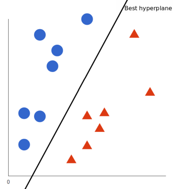Fig. 1. A simple SVM (Image Source: MonkeyLearn.com)

Consider the above image, with two sets of datapoints represented in blue circles and red traingles. SVM tries to learn the hyperplane which could divide these datapoints in two regions. As datapoints are 2 dimensional features (i.e. x & y), SVM learns 1 dimensional hyperplane which is a line.

To understand SVM completely, we need to go through and understand five concepts:

• Hyperplanes
• Marginal Distance
• Support Vector
• Linearly Separable
• Non Linear Separable

Hyperplanes

Hyperplanes are meant to be learnt by SVMs that divides the datapoints into two regions. Hyperplanes are n-dimensional where $n \in (1, \infty)$. Its dimensions are always 1 less than the dimensions of the dataset features. There are multiple viable hyperplanes which could divide the datapoints in two regions. Look at Fig. 2. which shows multiple possible hyperplanes.

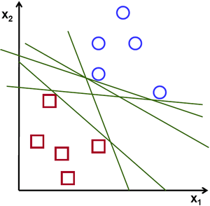Fig. 2. Multiple Possible Hyperplanes (Image Source: opencv.org)

Obviously, not any hyperplane can be selected as final hyperplane for the classification. SVM algorithm selects the best hyperplane which has maximum marginal distance with the closest data points of two classes.

Support Vector and Marginal Distance

Support Vectors are planes parallel to hyperplane that passes through atleast one data point of each class. Consider the fig. 3 below:

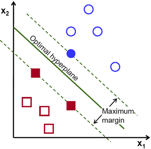Fig. 3. Lines parallel to ‘optimal hyperplane’ are support vectors

You could see a best hyperplane in center and there are two parallel hyperplanes to it. These are support vectors. These support vectors are passing through data points of each class. The distance between these two support vectors are called as marginal distance. SVM makes sure out of the many viable hyperlanes, the best selected hyperplanes has maximum marginal distance.

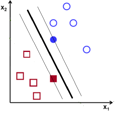Fig. 4. Alternative hyperplane and support vectors

In above fig. 4, there is another alternative hyperplane which divides the datapoints easily. But its support vectors has less marginal distance as compared to marginal distance in fig. 3. SVM would not select this set of hyperplanes but will select the hyperplanes in fig. 3.

Linearly and Non-Linearly Separable

The examples we’ve seen until now above have data which is linearly separable i.e. a line is sufficient to separate them. Real-world data rarely is linearly separable. Look at the data below in fig. 5. We couldn’t separate two set of data points by a line but on viewing we see datapoints are clearly separable. This is non-linear separable data.

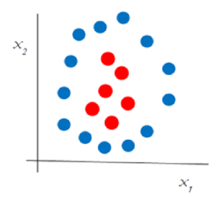Fig. 5. Non-linear data not separable (Image Source: mygreatlearning.com)

To segregate non-linear data, a third dimension is added. Until now we had only x and y dimesions, a third dimension z could be added with the help of a certain equation (for e.g. \z = x^{2} + y^{2}). This will give a three-dimensional space which could be easily sliceable by a 2 dimensional plane.

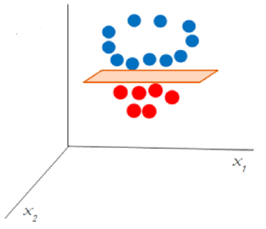Fig 6. Non-linear data becomes separable (Image Source: mygreatlearning.com)